Introduction
The classic n-Queens problem—placing n queens on an n×n chessboard so that no two queens attack each other—has long fascinated computer scientists and puzzle lovers alike. Even LinkedIn featured a Queens puzzle as an everyday challenge!
Many articles and posts have given ideas and codes for solving puzzles. However, building a puzzle game around n-Queens introduces a twist. It’s not just about solving the arrangement once. Instead, we need to generate distinct, playable “levels” for users, each with a unique solution or a limited number of solutions, plus additional constraints to make it fun and challenging.
This blog post will walk through how I’ve tackled that challenge:
- We’ll still solve the classic n-Queens puzzle—but randomly, to produce variety.
- We’ll then add colored regions so that each row, column, and colored region must have exactly one queen.
- Finally, we’ll show how to ensure each puzzle has an interesting structure and is solvable in a unique or near-unique way.
Note: You can play the game on my personal website.This article does not focus on the front-end or Django aspects. We’ll dive into the procedural generation algorithms behind the scenes, using Python, Cython, and a healthy dose of backtracking, flood fill, and multiprocessing.
Game Rules
The Board Layout
- One Queen Per Row: Each row on the chessboard must contain exactly one queen.
- One Queen Per Column: Each column must contain exactly one queen.
- One Queen Per Color Region: A board is divided into distinct colored regions, each of which may only contain one queen.
- No Attacks Allowed: Queens cannot attack each other—meaning no two queens share the same row, column, or diagonal.
Below is an example of a randomly generated valid 5×5 queens solution (before we add color constraints). Each queen is denoted with a red “Q.”

This basic arrangement is the familiar n-Queens problem on LeetCode. The difference comes next, when we break the board into color regions.
Procedural Puzzle Generation Algorithm
Let’s explore the puzzle generation in four main steps:
Step 1: Generate a Random Valid n-Queens Solution
Even though you might know a deterministic algorithm for n-Queens, it’s crucial to introduce randomness so that each puzzle is different. A straightforward way to do this is via randomized backtracking.
Below is a Cython-optimized snippet that shows the high-level idea:
cdef bint _backtrack(int row, int n, list solution,
                     object cols, object diag1, object diag2, list sol):
    if row == n:
        sol[0] = solution.copy()
        return True

    # Shuffle the columns for random exploration
    cdef list cols_list = list(range(n))
    random.shuffle(cols_list)

    for col in cols_list:
        # Check conflicts
        if col in cols or (row - col) in diag1 or (row + col) in diag2:
            continue

        # Place the queen
        solution[row] = col
        cols.add(col)
        diag1.add(row - col)
        diag2.add(row + col)

        # Recurse
        if _backtrack(row + 1, n, solution, cols, diag1, diag2, sol):
            return True

        # Backtrack
        cols.remove(col)
        diag1.remove(row - col)
        diag2.remove(row + col)

    return False

cpdef list random_n_queens(int n):
    cdef list solution = [None] * n
    ...
    _backtrack(0, n, solution, cols, diag1, diag2, sol)
    return sol[0]
- We maintain three sets (cols, diag1, and diag2) to quickly check if a spot conflicts with existing queens.
- For each row, we shuffle the columns. Randomizing column order speeds up “finding a random solution” because we effectively sample from the large solution space.
Once we have this valid arrangement, we proceed to color regions.
Step 2: Generate Color Regions (Region Partitioning)
The next challenge: ensure each colored region on the board also contains exactly one queen. We do this by:
- Seeding each region with exactly one queen’s position.
- Flood filling outward from each seed to color the rest of the board.
Below, we have an image that shows the board seeds: each queen’s cell is assigned a unique color (the rest are white).

We store region IDs in a 2D list, initially None except where the queen seeds are placed.
cpdef list generate_regions(int n, list queen_solution):
    cdef list regions = [[None for j in range(n)] for i in range(n)]
    # Shuffle region IDs so each puzzle is distinct
    cdef list region_ids = list(range(n))
    random.shuffle(region_ids)

    # Assign each queen’s row/column as an initial seed
    for i in range(n):
        rid = region_ids[i]
        r_seed = i
        c_seed = queen_solution[i]
        regions[r_seed][c_seed] = rid
    ...
    return regions
At this point, we have n seeds—one for each queen—and n region IDs.
Step 3: Expand Regions Using Flood Fill
Now we grow these seeded regions using a multi-source flood fill. Each region attempts to expand into adjacent, uncolored cells, with a random probability so that the final shapes vary.

Here is the relevant code snippet:
# Each region chooses a random expansion probability in [0.3, 0.5]
for rid in region_seeds:
    expansion_prob[rid] = 0.3 + 0.2 * random.random()

# Multi-source queue approach
for rid, seeds in region_seeds.items():
    for pos in seeds:
        queue.append((pos[0], pos[1], rid))

while queue:
    i, j, current_rid = queue.popleft()
    # Check adjacent cells
    for (di, dj) in [(-1,0),(1,0),(0,-1),(0,1)]:
        ni, nj = i+di, j+dj
        if 0 <= ni < n and 0 <= nj < n:
            if regions[ni][nj] is None:
                if random.random() < expansion_prob[current_rid]:
                    regions[ni][nj] = current_rid
                    queue.append((ni, nj, current_rid))
- We store a random expansion_prob[rid] for each region ID in [0.3, 0.5].
- In BFS fashion, each region tries to “capture” neighboring cells.
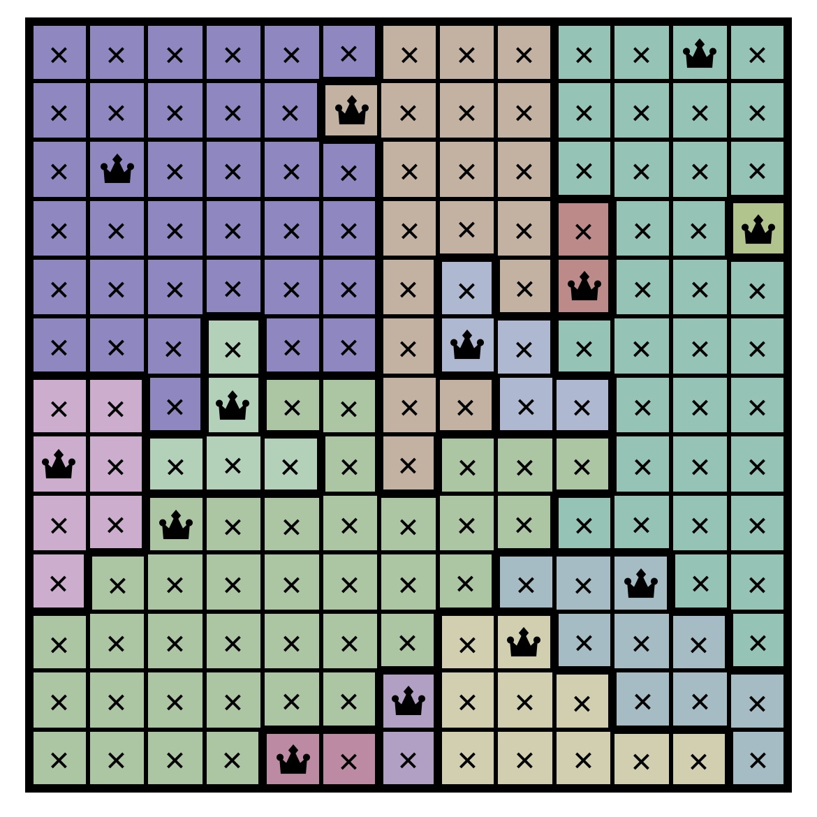
The result is a colorful mosaic where each region is connected, but the region sizes and boundaries vary from puzzle to puzzle.
Finally, we fill any leftover None cells by borrowing from adjacent region IDs, ensuring no cell remains uncolored.

Step 4: Validate the Puzzle for Uniqueness and Difficulty
At this point, we have an n-Queens arrangement and a color partition that demands exactly one queen per region. But how do we ensure the puzzle has a single solution or at least a limited number of solutions?
We do so by:
- Checking region connectivity (no isolated pockets).
- Running a specialized solver to count solutions up to the threshold of 1 for logical solvablility. If more solutions are found, we discard or re-generate.
We rely on a Cython + NumPy backtracking solver to verify solution counts:
def count_valid_solutions(object color_grid, int threshold):
    cdef int n = len(color_grid)
    cdef np.ndarray[DTYPE_t, ndim=2] arr = np.array(color_grid, dtype=np.intc)
    ...
    with nogil:
        result = _backtrack(0, n, 0, -100, grid_arr, threshold, used_blocks)
    return result
- We remove the Python GIL (with nogil) to maximize parallel performance.
- If result exceeds threshold, we stop exploring. This ensures we don’t waste time enumerating all solutions once we know the puzzle is “too easy.”
If the puzzle passes validation (region connectivity, limited solution count), we deem it a playable puzzle (the puzzle above is not playable with more than one solution).
Performance Challenges and Optimizations
Generating smaller puzzles (e.g., 4×4 up to 8×8) is straightforward. However, once you aim for n ≥ 14, it can take days to find enough unique puzzles that pass the single-solution test. Here’s how we tackle performance bottlenecks:
- Cython Speedups
- We compiled our backtracking and flood-fill code in Cython.
- We disabled GIL (nogil) in CPU-intensive loops to run them efficiently in C.
- NumPy Integration
- By converting color grids to NumPy arrays internally, we reduce overhead in checking adjacency, region membership, etc.
- Multiprocessing
- Puzzle generation can happen in parallel. We spawn multiple processes, each attempts to build a puzzle, and we combine unique ones that meet the difficulty criteria.
- Pruning
- Our solver stops the search early if it exceeds a solution threshold.
- The flood fill uses randomness, which helps us avoid exploring large swaths of similar puzzles.
Despite these optimizations, n=14 and above remains computationally expensive (it cost me 4 hours with a 32-core AMD 5950x for n=13). It’s still possible—but be prepared for long generation times!
Code Examples
Below are a few concise examples showing how we integrated Python and Cython:
1. Flood Fill in Cython
from collections import deque

cpdef list generate_regions(int n, list queen_solution):
    cdef list regions = [[None for j in range(n)] for i in range(n)]
    ...
    queue = deque()
    # ... Multi-source BFS in Cython ...
    return regions
2. Backtracking with Cython “nogil”
cdef int _backtrack(int row, int n, uint32_t used_cols, ... ) nogil:
    # Main logic for row-wise queen placement
    # 1) If row == n, return 1 solution
    # 2) For each col, check adjacency, region usage, etc.
    # 3) Recurse and prune if solutions exceed threshold
    ...
3. Parallel Generation
import multiprocessing

def worker_generate_map(n):
    new_map = generate_map(n)
    # Solve to check the puzzle’s solution count <= threshold
    solution = solve(new_map["colorGrid"], new_map["name"], threshold=1)
    if solution["number_solution"] <= 1:
        return new_map
    return None

if __name__ == '__main__':
    pool = multiprocessing.Pool()
    results = pool.map(worker_generate_map, [n] * batch_size)
    ...
Python vs. Cython Performance
- Pure Python backtracking is often tens to hundreds of times slower for large n (pure python cost me 24 hours for n=13 before I gave up).
- Cython with nogil can drastically improve throughput, especially when combined with multiprocessing.
- Memory layouts (e.g., contiguous NumPy arrays) also reduce overhead.
Real-World Applications in Game Design
The technique of randomly generating a valid puzzle, then layering constraints is widely used in puzzle and game design. Notable examples include:
- Sudoku Generation – Randomly assign digits, then prune puzzles to ensure they have a unique solution.
- Maze Generation – Carve passages via random DFS or randomized Kruskal’s algorithm, then ensure the maze structure is solvable.
- AI-Driven Puzzle Creation – Use search or machine learning to produce “fun” puzzle variants at scale.
Future Directions
- Machine Learning for Difficulty Tuning: Train a model that predicts puzzle difficulty from partial constraints, then “reject” easy or overly hard puzzles mid-generation.
- “Trap Puzzles”: Generate boards that appear solvable but have no valid solutions once certain constraints are applied—players must discover a contradiction.
Conclusion
Designing a puzzle game from the n-Queens problem requires more than just finding a solution—it demands a robust procedural generation pipeline that ensures uniqueness, difficulty control, and an engaging experience for players. Our approach incorporates:
- Randomized n-Queens backtracking to diversify solutions.
- Region-based constraints enforced by flood fill.
- Cython + NumPy + multiprocessing for performance.
- Validation to ensure each puzzle is solvable (but not too solvable!).
The complete codes can be found on my github. If you’re intrigued by how AI or advanced heuristics might push puzzle-generation boundaries, or if you have feedback on these algorithms, let’s connect. This is an exciting space where puzzle-solving meets code optimization and game design innovation.
Thank you for reading, and I look forward to any discussions, pull requests, or collaborations!